
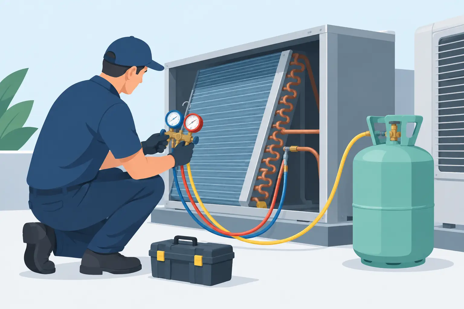
A refrigerant charge estimate is not a nameplate calculation. For a DX system, the installed charge is the refrigerant inventory required to support a specific operating condition across the evaporator, condenser, interconnecting lines, receiver, and accessory components. To estimate refrigerant charge with engineering usefulness, the calculation must account for local refrigerant state and density rather than treating every internal volume as liquid-filled.
This distinction matters most during equipment development, coil selection, system optimization, and design validation. An understated charge estimate can produce inadequate receiver capacity, poor low-ambient behavior, or an evaporator starved during transients. An overstated estimate can obscure charge-reduction opportunities and create avoidable cost, regulatory, and safety exposure.
Define What the Charge Estimate Must Represent
Before calculating mass, define the system boundary and the operating state. A factory charge, a running charge, a pump-down inventory, and a maximum flooded-receiver condition are not interchangeable values.
For a packaged refrigeration system, the boundary may include the compressor shell, condenser, liquid line, filter-drier, receiver, expansion device, evaporator, suction line, and accumulator. For an OEM coil analysis, the immediate concern may be the refrigerant held in the condenser and evaporator circuits only. Both are valid applications, but they answer different questions.
The operating point is equally important. Refrigerant density in a condenser circuit changes substantially between a high-load condition with a short subcooled region and a low-ambient condition where liquid backs up into the coil. The evaporator inventory also changes with superheat setting, distributor behavior, circuit balance, and load. A single charge value without a stated condition should be treated as a preliminary planning number, not a design result.
Estimate Refrigerant Charge by Component Volume
The fundamental relationship is straightforward:
\[ m = \rho V \]
where mass, m, equals refrigerant density, ρ, multiplied by internal volume, V. The engineering work lies in assigning the appropriate volume and density to each region of the system.
A useful component-level estimate separates the inventory into condenser, receiver, liquid line, expansion device and distributor, evaporator, suction line, compressor, and any accumulator or oil-management hardware. Each component should be evaluated at its expected pressure, temperature, and phase condition.
For a single-phase liquid region, the calculation is relatively direct. Determine the internal volume and multiply it by liquid density at the relevant liquid temperature. For a suction line or superheated evaporator outlet, use vapor density at the local suction pressure and temperature. Those values can differ by orders of magnitude, which is why substituting one average density for the entire system creates large errors.
Two-phase regions require more care. A DX evaporator circuit, for example, contains a changing mixture density from the distributor inlet through the boiling region and into the superheated outlet section. The condenser has desuperheating, two-phase condensation, and subcooling regions. Assigning saturated liquid density to the full coil volume will overpredict charge. Assigning a uniform quality to the entire coil can be just as misleading.
Divide Coils Into Thermodynamic Regions
For preliminary work, divide each coil circuit into regions with distinct refrigerant states. In a condenser, these are commonly the superheated vapor region, saturated two-phase region, and subcooled liquid region. In a DX evaporator, use a two-phase boiling region and a superheated vapor region, with additional segmentation if pressure drop or temperature glide warrants it.
Calculate the mass of each segment as:
\[ m_i = \rho_i V_i \]
Then sum the segment inventories. The accuracy of this method depends on the quality of the predicted region lengths, local pressure drop, and refrigerant properties. It is far more defensible than applying a coil-level average density.
For zeotropic blends, evaluate properties at the applicable local composition and saturation condition. Bubble and dew temperatures are not interchangeable. Condensing and evaporating pressure drop also changes local saturation temperature and density, particularly in long circuits or high-capacity coils.
Engineering-grade thermal analysis is valuable here because it predicts how circuit geometry, airflow, capacity, refrigerant selection, and operating conditions distribute the two-phase and single-phase regions. Charge is then derived from the modeled thermal state rather than assumed from nominal capacity alone.
Start With Accurate Internal Volumes
A charge calculation cannot be more accurate than the volume data behind it. Tube inside diameter, effective tube length, number of parallel circuits, return bends, headers, distributors, and connection tubes all contribute. Small omissions are cumulative, especially in compact systems with low total charge targets.
Tube volume should be based on actual inside diameter, not nominal tube size. For a straight circular tube:
\[ V = \frac{\pi D_i^2}{4}L \]
where Dᵢ is inside diameter and L is developed length. Include return bends using centerline length or supplier geometry. Header and manifold volumes should come from drawings, CAD data, or direct measurement. Do not infer them from tube volume ratios when the receiver, headers, or suction accumulator represent a meaningful share of total inventory.
Accessories can be material contributors. A liquid receiver may intentionally contain most of the adjustable system inventory. An accumulator, oil separator, liquid-line heat exchanger, sight glass, or large filter-drier can also affect the charge balance. Their state may vary by operating condition, so their maximum and normal inventories should be evaluated separately.
Account for System Conditions That Move Charge
Charge distribution is dynamic. The total mass in a sealed system is fixed, but the mass held in any component moves as condensing pressure, evaporating pressure, load, fan control, and ambient conditions change.
At low ambient, a head-pressure control strategy may flood condenser volume with liquid. The condenser inventory rises while receiver inventory falls. A charge sized only at a high-ambient rating condition may therefore be inadequate for stable low-ambient operation.
During pull-down or after a defrost event, evaporator and suction-line inventory can increase temporarily. Compressor cycling, variable-speed compression, electronic expansion valve control, and hot-gas defrost create further shifts. For systems with tight charge margins, evaluate more than one steady-state point and identify the condition that produces the lowest usable receiver level and the condition that produces the highest liquid inventory.
The receiver is not simply a storage vessel added after the coil calculation. It is the component that absorbs system inventory changes while preserving a solid liquid supply to the expansion device. Its required volume depends on charge migration, allowable fill fraction, and the specific operating envelope. A receiver that appears adequate at design ambient may be undersized during low-ambient flooding or pump-down.
Use Coil Modeling to Reduce Assumptions
Capacity-based charge rules can be useful for early feasibility estimates, but they do not capture geometry-dependent inventory. Two coils with identical nominal capacity can have substantially different charge because of tube diameter, circuit count, face area, circuit length, distributor design, and subcooling requirement.
A thermal model provides a better basis by calculating refrigerant-side pressure drop, heat transfer, phase-region distribution, and outlet condition across each circuit. From that result, the coil inventory can be integrated segment by segment. This is particularly relevant when comparing microchannel and round-tube condensers, optimizing circuit layouts, or changing refrigerants.
ExCoil supports this type of engineering workflow for DX evaporator and condenser analysis: evaluate the coil thermal behavior first, then use the predicted refrigerant state distribution to support a charge estimate. The resulting value remains an estimate until system-level validation, but it is grounded in the conditions that actually determine coil inventory.
Validate the Estimate Against Hardware
The final charge must be confirmed on representative hardware. Manufacturing variation in tube length, header fabrication, oil retention, piping routing, and accessory selection can shift the installed inventory. Field piping can dominate the difference between a unit-level calculation and an installed-system charge.
Validation should compare predicted and measured performance at the critical operating conditions identified during design. Confirm liquid availability at the expansion device, receiver level where applicable, evaporator superheat control, condenser subcooling, and system response across ambient and load changes. If measured behavior differs from the model, isolate whether the cause is volume, refrigerant property assumptions, pressure drop, control behavior, or an unmodeled component.
A charge estimate earns its value when it clarifies design decisions before prototype testing, not when it substitutes for testing. Build the estimate from component volumes and local thermodynamic states, evaluate the operating envelope, and use test data to close the remaining uncertainty.